-
transformer(deepseek)
Thinking…
Transformers are a type of neural network architecture introduced in the paper “Attention Is All You Need” by Vaswani et al. in 2017. They revolutionized NLP tasks. Unlike previous models like RNNs or LSTMs, Transformers use self-attention mechanisms to process all words in a sequence simultaneously, allowing for more parallelization and handling long-range dependencies better.
I should explain the key components: self-attention, multi-head attention, positional encoding, encoder-decoder structure. Also, mention the impact of Transformers on models like BERT, GPT, T5, etc. It’s important to highlight their advantages over RNNs and why they became so popular.
Wait, the user might be looking for both a basic explanation and maybe some details on how they work. Let me structure this logically. Start with an overview, then key components, how they work, advantages, applications, and popular models. That should cover the essentials.
I need to make sure the explanation of self-attention is clear. Maybe use an example, like how each word relates to others in a sentence. Also, touch on positional encoding since Transformers don’t have inherent sequence order understanding like RNNs.
Oh, and the user might be interested in knowing that Transformers are used beyond NLP now, in areas like computer vision with Vision Transformers. Applications are important to mention too—machine translation, text generation, etc.
I should check if there are any common confusions to address. For example, the difference between the Transformer architecture and the models built on it, like BERT vs. the original Transformer. Also, maybe mention the computational aspects, like the need for large datasets and resources.
Make sure the answer is comprehensive but not too technical. Use bullet points for clarity. Alright, time to put it all together in a structured way.
Thinking…Transformers in Deep Learning
Transformers are a groundbreaking neural network architecture introduced in the 2017 paper Attention Is All You Need. They revolutionized natural language processing (NLP) and are now widely used in tasks like translation, text generation, and more. Here’s a breakdown:
Key Components
- Self-Attention Mechanism
- Allows the model to weigh the importance of different words in a sequence relative to each other.
- Example: In “The cat sat on the mat,” the word “cat” relates strongly to “sat” and “mat.”
- Multi-Head Attention
- Runs multiple self-attention operations in parallel, capturing diverse relationships (e.g., syntax, semantics).
- Positional Encoding
- Injects information about word order into the model (since Transformers process sequences in parallel, unlike RNNs).
- Feed-Forward Networks
- Applies non-linear transformations to individual positions after attention.
- Encoder-Decoder Architecture
- Encoder: Processes input and builds contextual representations.
- Decoder: Generates output (e.g., translated text) using encoder outputs and previous decoder states.
How Transformers Work
- Input Embedding: Convert input tokens (words/subwords) into vectors.
- Add Positional Encoding: Embed positional information into vectors.
- Self-Attention Layer: Compute relationships between all tokens.
- Feed-Forward Layer: Refine representations.
- Repeat: Stack multiple layers to capture deeper patterns.
Advantages Over RNNs/CNNs
- Parallelization: Processes entire sequences at once (faster training).
- Long-Range Dependencies: Handles relationships between distant tokens better (no sequential decay).
- Scalability: Efficiently trained on massive datasets (e.g., GPT-3 with 175B parameters).
Applications
- Language Models: GPT, BERT, T5.
- Machine Translation: Google Translate.
- Text Generation: ChatGPT, Claude.
- Vision: Vision Transformers (ViT) for image classification.
- Multimodal Tasks: Models like DALL·E (text-to-image).
Popular Transformer Models
Model Type Use Case BERT Encoder-only Text classification, QA GPT Decoder-only Text generation T5 Encoder-Decoder Text-to-text tasks ViT Vision Image classification
Challenges
- Computational Cost: Requires massive compute/resources (e.g., GPT-4).
- Context Length: Limited by attention’s quadratic complexity (fixed in variants like Flash Attention).
Transformers have become the backbone of modern AI, pushing the boundaries of what’s possible in NLP, vision, and beyond. Let me know if you’d like a deeper dive into any aspect! 🤖
-
卷积神经网络(DeepSeeK)
Thinking…
卷积神经网络(Convolutional Neural Network,CNN)是一种深度学习模型,专门用于处理具有网格结构的数据(如图像、视频、音频等)。其核心思想是通过局部感知、权重共享和空间下采样来自动提取数据中的层次化特征。
以下是卷积神经网络的核心组件和工作原理:
1. 核心组件(1) 卷积层(Convolutional Layer)
- 功能:通过卷积核(滤波器)扫描输入数据,提取局部特征(如边缘、纹理等)。
- 操作:
- 输入数据(如RGB图像)与卷积核进行滑动窗口点乘。
- 输出特征图(Feature Map),反映输入中特定模式的存在位置。
- 参数:
- 卷积核大小(如3×3)、步长(Stride)、填充(Padding)。
(2) 激活函数(Activation Function)
- 作用:引入非线性,增强模型表达能力。
- 常用函数:ReLU(Rectified Linear Unit)、Sigmoid、Leaky ReLU。
(3) 池化层(Pooling Layer)
- 功能:降低特征图的空间维度,减少计算量并增强模型鲁棒性。
- 操作:
- 最大值池化(Max Pooling):取局部区域最大值。
- 平均值池化(Average Pooling):取局部区域平均值。
(4) 全连接层(Fully Connected Layer)
- 功能:将提取的特征映射到最终输出(如分类结果)。
- 特点:每个神经元与前一层的所有神经元连接。
2. 经典CNN架构
(1) LeNet-5
- 提出者:Yann LeCun(1998)。
- 应用:手写数字识别(MNIST)。
- 结构:卷积层 → 池化层 → 卷积层 → 池化层 → 全连接层。
(2) AlexNet
- 里程碑:2012年ImageNet竞赛冠军,开启了深度学习热潮。
- 改进:
- 使用ReLU激活函数加速训练。
- 引入Dropout防止过拟合。
- 多GPU并行训练。
(3) VGGNet
- 特点:通过堆叠小卷积核(3×3)代替大卷积核,减少参数并增强非线性。
(4) ResNet
- 创新:残差学习(Residual Learning),通过跳跃连接(Skip Connection)解决深层网络梯度消失问题。
- 效果:可训练超过1000层的网络。
3. CNN的优势
- 自动特征提取:无需手动设计特征,适合处理高维数据。
- 平移不变性:通过卷积和池化操作,对输入的小幅位移具有鲁棒性。
- 参数共享:同一卷积核在输入的不同位置重复使用,减少参数量。
4. 应用场景
- 图像分类(如识别猫狗)。
- 目标检测(如YOLO、Faster R-CNN)。
- 语义分割(如U-Net)。
- 图像生成(如生成对抗网络GAN)。
- 自然语言处理(如文本分类)。
5. 代码示例(PyTorch)
import torch
import torch.nn as nn

class SimpleCNN(nn.Module):
    def __init__(self):
        super(SimpleCNN, self).__init__()
        self.conv1 = nn.Conv2d(3, 16, 3)  # 输入通道3,输出通道16,卷积核3×3
        self.pool = nn.MaxPool2d(2, 2)    # 池化层2×2
        self.fc = nn.Linear(16*16*16, 10) # 全连接层(假设输入图像为32×32)

    def forward(self, x):
        x = self.pool(nn.functional.relu(self.conv1(x))) # 卷积 → ReLU → 池化
        x = x.view(-1, 16*16*16)          # 展平特征图
        x = self.fc(x)
        return x

model = SimpleCNN()
6. 挑战与改进
- 过拟合:通过数据增强、Dropout、正则化缓解。
- 计算资源需求:使用轻量化模型(如MobileNet、ShuffleNet)。
- 可解释性:通过类激活图(CAM)、梯度可视化等方法分析模型决策。
卷积神经网络是计算机视觉领域的基石,理解其原理和实现方式是掌握深度学习的关键!
-
Native Sparse Attention Hardware-Aligned and NativelyTrainable Sparse Attention
-
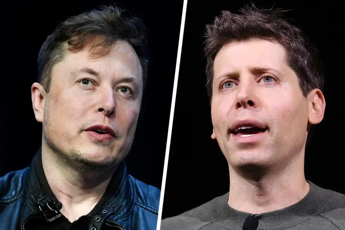
20万张GPU!号称“地球上最聪明的AI”Grok-3来了,斩获多个Top1
北京时间 2 月 18 日中午,埃隆·马斯克旗下的人工智能公司 xAI 重磅发布了 Grok 3 系列模型,宣称其在数学、科学和编码基准测试中,击败了 Google Gemini、DeepSeek V3、Claude 以及 OpenAI 的 GPT-4o。
更为值得关注的是,Grok 3 的训练并非如此前传闻的在“10 万张 GPU 上进行”,而是使用了“20 万张 GPU”。对此,有网友指出其算力消耗是 DeepSeek V3 的 263 倍。正因此,“又壕又横”的马斯克将其称为“地球上最聪明的 AI”。
Grok 3 基准测试曝光根据 xAI 工程师的介绍,Grok 3 其实是一个模型家族——而不仅仅是一个模型。Grok 3 的轻量级版本——Grok 3 mini——在牺牲一定准确度的情况下,能够更快地响应问题。
目前,并不是所有模型都已经上线(其中一些仍处于测试阶段),但会从今天开始陆续推出。此外,原定今天要发布的语音模式并未出现,马斯克随后也在 X 上解释称,“语言模式仍然有点不完善,所以大概会在一周左右推出,但它很棒。”
根据官方公开的测试结果,Grok 3 在包括 AIME(评估模型在一系列数学问题上的表现)和 GPQA(评估模型在博士级别的物理学、生物学和化学问题上的表现)等基准测试中,远超 GPT-4o、Gemini-2 Pro、DeepSeek V3、Claude 3.5 Sonnet 等大模型。
在大模型竞技场 Chatbot Arena(LMSYS)测试中,xAI 工程师表示,早期版本的 Grok-3 获得了第一的成绩,达到了 1402 分,超越了 Gemini 2.0 Flash Thinking 实验版本、ChatGPT-4o 最新版本以及最近大火的 DeepSeek R1 等等。要知道在 Chatbot Arena 中,用户或评审可以通过对比不同的模型响应,并进行投票,以评定哪个模型提供了最佳的答案。平台通过这种“人类评分”的方式帮助研究人员和开发者了解各大聊天机器人模型的优劣,推动模型的持续改进。时下 Grok 3 是在过往业界已发布的大模型中首个突破 1400 分、获得多个第一的大模型。
-
机器学习十大算法
机器学习十大算法的 Python 代码示例,我们将使用常见的
scikit-learn库来实现,数据集使用鸢尾花数据集。1. 决策树算法(Decision Tree)
from sklearn.datasets import load_iris
from sklearn.model_selection import train_test_split
from sklearn.tree import DecisionTreeClassifier
from sklearn.metrics import accuracy_score

# 加载数据集
iris = load_iris()
X = iris.data
y = iris.target

# 划分训练集和测试集
X_train, X_test, y_train, y_test = train_test_split(X, y, test_size=0.3, random_state=42)

# 创建决策树分类器
clf = DecisionTreeClassifier()
clf.fit(X_train, y_train)

# 预测
y_pred = clf.predict(X_test)

# 计算准确率
accuracy = accuracy_score(y_test, y_pred)
print(f"决策树准确率: {accuracy}")
2. 朴素贝叶斯算法(Naive Bayes)
from sklearn.datasets import load_iris
from sklearn.model_selection import train_test_split
from sklearn.naive_bayes import GaussianNB
from sklearn.metrics import accuracy_score

# 加载数据集
iris = load_iris()
X = iris.data
y = iris.target

# 划分训练集和测试集
X_train, X_test, y_train, y_test = train_test_split(X, y, test_size=0.3, random_state=42)

# 创建朴素贝叶斯分类器
clf = GaussianNB()
clf.fit(X_train, y_train)

# 预测
y_pred = clf.predict(X_test)

# 计算准确率
accuracy = accuracy_score(y_test, y_pred)
print(f"朴素贝叶斯准确率: {accuracy}")
3. 支持向量机(Support Vector Machine,SVM)
from sklearn.datasets import load_iris
from sklearn.model_selection import train_test_split
from sklearn.svm import SVC
from sklearn.metrics import accuracy_score

# 加载数据集
iris = load_iris()
X = iris.data
y = iris.target

# 划分训练集和测试集
X_train, X_test, y_train, y_test = train_test_split(X, y, test_size=0.3, random_state=42)

# 创建 SVM 分类器
clf = SVC()
clf.fit(X_train, y_train)

# 预测
y_pred = clf.predict(X_test)

# 计算准确率
accuracy = accuracy_score(y_test, y_pred)
print(f"SVM 准确率: {accuracy}")
4. K 近邻算法(K – Nearest Neighbor,KNN)
from sklearn.datasets import load_iris
from sklearn.model_selection import train_test_split
from sklearn.neighbors import KNeighborsClassifier
from sklearn.metrics import accuracy_score

# 加载数据集
iris = load_iris()
X = iris.data
y = iris.target

# 划分训练集和测试集
X_train, X_test, y_train, y_test = train_test_split(X, y, test_size=0.3, random_state=42)

# 创建 KNN 分类器
clf = KNeighborsClassifier()
clf.fit(X_train, y_train)

# 预测
y_pred = clf.predict(X_test)

# 计算准确率
accuracy = accuracy_score(y_test, y_pred)
print(f"KNN 准确率: {accuracy}")
5. 逻辑回归(Logistic Regression)
from sklearn.datasets import load_iris
from sklearn.model_selection import train_test_split
from sklearn.linear_model import LogisticRegression
from sklearn.metrics import accuracy_score

# 加载数据集
iris = load_iris()
X = iris.data
y = iris.target

# 划分训练集和测试集
X_train, X_test, y_train, y_test = train_test_split(X, y, test_size=0.3, random_state=42)

# 创建逻辑回归分类器
clf = LogisticRegression(max_iter=1000)
clf.fit(X_train, y_train)

# 预测
y_pred = clf.predict(X_test)

# 计算准确率
accuracy = accuracy_score(y_test, y_pred)
print(f"逻辑回归准确率: {accuracy}")
6. 随机森林算法(Random Forest)
from sklearn.datasets import load_iris
from sklearn.model_selection import train_test_split
from sklearn.ensemble import RandomForestClassifier
from sklearn.metrics import accuracy_score

# 加载数据集
iris = load_iris()
X = iris.data
y = iris.target

# 划分训练集和测试集
X_train, X_test, y_train, y_test = train_test_split(X, y, test_size=0.3, random_state=42)

# 创建随机森林分类器
clf = RandomForestClassifier()
clf.fit(X_train, y_train)

# 预测
y_pred = clf.predict(X_test)

# 计算准确率
accuracy = accuracy_score(y_test, y_pred)
print(f"随机森林准确率: {accuracy}")
7. 梯度提升树(Gradient Boosting Decision Tree,GBDT)
from sklearn.datasets import load_iris
from sklearn.model_selection import train_test_split
from sklearn.ensemble import GradientBoostingClassifier
from sklearn.metrics import accuracy_score

# 加载数据集
iris = load_iris()
X = iris.data
y = iris.target

# 划分训练集和测试集
X_train, X_test, y_train, y_test = train_test_split(X, y, test_size=0.3, random_state=42)

# 创建 GBDT 分类器
clf = GradientBoostingClassifier()
clf.fit(X_train, y_train)

# 预测
y_pred = clf.predict(X_test)

# 计算准确率
accuracy = accuracy_score(y_test, y_pred)
print(f"GBDT 准确率: {accuracy}")
8. K – 均值聚类算法(K – Means Clustering)
from sklearn.datasets import load_iris
from sklearn.cluster import KMeans
import matplotlib.pyplot as plt

# 加载数据集
iris = load_iris()
X = iris.data

# 创建 KMeans 聚类器
kmeans = KMeans(n_clusters=3, random_state=42)
kmeans.fit(X)

# 获取聚类标签
labels = kmeans.labels_

# 可视化聚类结果(取前两个特征)
plt.scatter(X[:, 0], X[:, 1], c=labels, cmap='viridis')
centers = kmeans.cluster_centers_
plt.scatter(centers[:, 0], centers[:, 1], c='red', marker='X', s=200)
plt.title('K - Means Clustering')
plt.xlabel('Sepal length')
plt.ylabel('Sepal width')
plt.show()
9. 主成分分析(Principal Component Analysis,PCA)
from sklearn.datasets import load_iris
from sklearn.decomposition import PCA
import matplotlib.pyplot as plt

# 加载数据集
iris = load_iris()
X = iris.data

# 创建 PCA 对象,降维到 2 维
pca = PCA(n_components=2)
X_pca = pca.fit_transform(X)

# 可视化降维后的数据
plt.scatter(X_pca[:, 0], X_pca[:, 1], c=iris.target, cmap='viridis')
plt.title('PCA of Iris Dataset')
plt.xlabel('Principal Component 1')
plt.ylabel('Principal Component 2')
plt.show()
10. AdaBoost 算法(Adaptive Boosting)
from sklearn.datasets import load_iris
from sklearn.model_selection import train_test_split
from sklearn.ensemble import AdaBoostClassifier
from sklearn.metrics import accuracy_score

# 加载数据集
iris = load_iris()
X = iris.data
y = iris.target

# 划分训练集和测试集
X_train, X_test, y_train, y_test = train_test_split(X, y, test_size=0.3, random_state=42)

# 创建 AdaBoost 分类器
clf = AdaBoostClassifier()
clf.fit(X_train, y_train)

# 预测
y_pred = clf.predict(X_test)

# 计算准确率
accuracy = accuracy_score(y_test, y_pred)
print(f"AdaBoost 准确率: {accuracy}")
这些代码示例展示了如何使用
scikit-learn库实现机器学习十大算法,并在鸢尾花数据集上进行简单的训练和测试。你可以根据实际需求调整参数和使用其他数据集。 -
K-Means 算法
K-Means 是一种无监督学习算法,用于将数据点划分为
k个不同的簇。下面是使用 PyTorch 实现 K-Means 算法的代码示例:import torch def kmeans(X, k, max_iter=100): """ K-Means 算法的 PyTorch 实现 参数: X (torch.Tensor): 输入数据,形状为 (n_samples, n_features) k (int): 簇的数量 max_iter (int): 最大迭代次数 返回: torch.Tensor: 每个数据点所属的簇的索引 torch.Tensor: 每个簇的中心点 """ # 随机初始化中心点 n_samples, n_features = X.shape indices = torch.randperm(n_samples)[:k] centroids = X[indices] for _ in range(max_iter): # 计算每个数据点到每个中心点的距离 distances = torch.cdist(X, centroids) # 找到每个数据点最近的中心点 labels = torch.argmin(distances, dim=1) # 更新中心点 new_centroids = torch.zeros(k, n_features, dtype=X.dtype, device=X.device) for i in range(k): cluster_points = X[labels == i] if len(cluster_points) > 0: new_centroids[i] = torch.mean(cluster_points, dim=0) else: # 如果某个簇为空,重新随机初始化该中心点 new_centroids[i] = X[torch.randint(0, n_samples, (1,))] # 判断是否收敛 if torch.allclose(centroids, new_centroids): break centroids = new_centroids return labels, centroids你可以使用以下方式调用这个函数:
# 生成一些示例数据
n_samples = 100
n_features = 2
X = torch.randn(n_samples, n_features)

# 运行 K-Means 算法
k = 3
labels, centroids = kmeans(X, k)

print("每个数据点所属的簇的索引:", labels)
print("每个簇的中心点:", centroids)
代码解释:
- 初始化中心点:从输入数据中随机选择
k个点作为初始中心点。 - 迭代更新:
- 计算每个数据点到每个中心点的距离。
- 找到每个数据点最近的中心点,并将其分配到该簇。
- 更新每个簇的中心点,即计算该簇中所有数据点的平均值。
- 收敛判断:如果中心点不再发生变化,则认为算法收敛,停止迭代。
注意事项:
- 该实现使用欧几里得距离来计算数据点之间的距离。
- 如果某个簇为空,我们重新随机初始化该簇的中心点,以避免出现中心点为零向量的情况。
- 初始化中心点:从输入数据中随机选择
-
Happy Valentine’s Day!


您可能也喜欢

花花草草治愈人心
-
974亿!马斯克出手收购OpenAI

据美国《华尔街日报》10日报道,代理律师当天表示,世界首富、美国亿万富翁埃隆·马斯克带领一群投资者,出资970亿美元寻求收购控制人工智能(AI)公司OpenAI的非营利组织。该交易达成后,马斯克会让OpenAI与他旗下的人工智能公司xAI合并。
报道称,目前,马斯克与OpenAI首席执行官萨姆·奥尔特曼正在就OpenAI的未来方向和控制权打官司,这起收购案将使奥尔特曼为该公司制定的计划变得更加复杂,其中包括将其改造成一家营利性公司,以及参与白宫不久前宣布的一项名为“星际之门”(Stargate)的AI项目。据称,该项目将为美国人工智能基础设施投资高达5000亿美元。
马斯克通过律师发表声明称:“是时候让OpenAI回归开源,恢复成它曾经是的那种注重安全的向善力量了。我们将确保这一点。”
不过,马斯克的收购请求遭到奥尔特曼迅速拒绝。当地时间10日,奥尔特曼在社交平台X上回应称:“不了,谢谢,不过如果你愿意的话,我们将出资97.4亿美元收购推特(Twitter)。”2022年,马斯克收购社交平台推特后将其改名为“X”。美媒注意到,奥尔特曼的出价刚好是马斯克出价的十分之一。随后,马斯克在奥尔特曼的这一帖子下面评论称:“骗子”。
同一天,奥尔特曼还向OpenAI工作人员发表公开信称:“我们的组织结构确保没有任何个人可以控制OpenAI……(马斯克的收购要约)是试图削弱我们的策略,因为我们正在取得巨大进步。”
报道称,马斯克和奥尔特曼均是OpenAI的联合创始人,两人在2015年共同创立的OpenAI最初是一个非营利研究机构。2019年,在马斯克离开后,奥尔特曼成为首席执行官。2022年,OpenAI推出人工智能对话机器人ChatGPT,引发广泛关注。
在奥尔特曼的领导下,OpenAI设立了一家营利性子公司,目的是吸引投资。目前,奥尔特曼正在将OpenAI改造成一家营利性公司。
-
春天来了
您可能也喜欢
花花草草治愈人心
-
知识蒸馏(Knowledge Distillation)
知识蒸馏(Knowledge Distillation)是一种模型压缩和迁移学习的技术,通过将一个大型的、性能较好的教师模型(Teacher Model)的知识传递给一个小型的学生模型(Student Model),从而使学生模型能够在保持较高性能的同时减少计算资源和内存的使用。下面是一个使用 PyTorch 在 MNIST 数据集上进行知识蒸馏的示例代码:
import torch
import torch.nn as nn
import torch.optim as optim
from torchvision import datasets, transforms
from torch.utils.data import DataLoader

# 定义教师模型
class TeacherModel(nn.Module):
    def __init__(self):
        super(TeacherModel, self).__init__()
        self.fc1 = nn.Linear(784, 128)
        self.fc2 = nn.Linear(128, 64)
        self.fc3 = nn.Linear(64, 10)

    def forward(self, x):
        x = x.view(-1, 784)
        x = torch.relu(self.fc1(x))
        x = torch.relu(self.fc2(x))
        x = self.fc3(x)
        return x

# 定义学生模型
class StudentModel(nn.Module):
    def __init__(self):
        super(StudentModel, self).__init__()
        self.fc1 = nn.Linear(784, 32)
        self.fc2 = nn.Linear(32, 10)

    def forward(self, x):
        x = x.view(-1, 784)
        x = torch.relu(self.fc1(x))
        x = self.fc2(x)
        return x

# 数据预处理
transform = transforms.Compose([
    transforms.ToTensor(),
    transforms.Normalize((0.1307,), (0.3081,))
])

# 加载 MNIST 数据集
train_dataset = datasets.MNIST(root='./data', train=True,
                               download=True, transform=transform)
test_dataset = datasets.MNIST(root='./data', train=False,
                              download=True, transform=transform)

train_loader = DataLoader(train_dataset, batch_size=64, shuffle=True)
test_loader = DataLoader(test_dataset, batch_size=64, shuffle=False)

# 训练教师模型
teacher_model = TeacherModel()
criterion = nn.CrossEntropyLoss()
optimizer = optim.Adam(teacher_model.parameters(), lr=0.001)

for epoch in range(5):
    running_loss = 0.0
    for i, (images, labels) in enumerate(train_loader):
        optimizer.zero_grad()
        outputs = teacher_model(images)
        loss = criterion(outputs, labels)
        loss.backward()
        optimizer.step()
        running_loss += loss.item()
    print(f'Epoch {epoch + 1}, Loss: {running_loss / len(train_loader)}')

# 知识蒸馏
student_model = StudentModel()
optimizer_student = optim.Adam(student_model.parameters(), lr=0.001)
temperature = 2.0
alpha = 0.5

for epoch in range(5):
    running_loss = 0.0
    for i, (images, labels) in enumerate(train_loader):
        optimizer_student.zero_grad()

        # 教师模型输出
        teacher_outputs = teacher_model(images)
        teacher_logits = teacher_outputs / temperature
        teacher_probs = torch.softmax(teacher_logits, dim=1)

        # 学生模型输出
        student_outputs = student_model(images)
        student_logits = student_outputs / temperature
        student_probs = torch.softmax(student_logits, dim=1)

        # 蒸馏损失
        distillation_loss = nn.KLDivLoss(reduction='batchmean')(torch.log(student_probs), teacher_probs) * (temperature ** 2)

        # 学生模型与真实标签的交叉熵损失
        student_loss = nn.CrossEntropyLoss()(student_outputs, labels)

        # 总损失
        total_loss = alpha * distillation_loss + (1 - alpha) * student_loss

        total_loss.backward()
        optimizer_student.step()
        running_loss += total_loss.item()

    print(f'Epoch {epoch + 1}, Student Loss: {running_loss / len(train_loader)}')

# 测试学生模型
correct = 0
total = 0
with torch.no_grad():
    for images, labels in test_loader:
        outputs = student_model(images)
        _, predicted = torch.max(outputs.data, 1)
        total += labels.size(0)
        correct += (predicted == labels).sum().item()

print(f'Accuracy of the student network on the 10000 test images: {100 * correct / total}%')
代码说明:
- 模型定义:定义了一个简单的三层全连接教师模型和一个两层全连接学生模型。
- 数据加载:使用
torchvision加载 MNIST 数据集,并进行预处理。 - 教师模型训练:使用交叉熵损失函数和 Adam 优化器训练教师模型。
- 知识蒸馏:使用 KL 散度损失函数计算教师模型和学生模型输出的软标签之间的损失,同时结合学生模型与真实标签的交叉熵损失,得到总损失。
- 学生模型测试:在测试集上评估学生模型的准确率。
通过知识蒸馏,学生模型可以从教师模型中学习到更多的知识,从而提高性能。